Session 1

Introduction to R and R Commander (Rcmdr) and R functions for basic statistical models (L611)

Topic 1 (Installation / R Graphics)
- Installations
- Graphics in R
Topic 2 (Descriptive Stats / Probability)
- Symmetry, positively-skewed and negatively-skewed
- Mean and variance of a dataset
- Probability calculations
Topic 3 (Random Variables)
- Discrete random variables
- Binomial (a special discrete random variable)
- Normal (a special continuous random variable)
- An important example (Roulette)
Topic 4 (Confidence Intervals / Hypothesis Testing)
- Confidence intervals
- Hypothesis testing (and Type I and Type II errors)

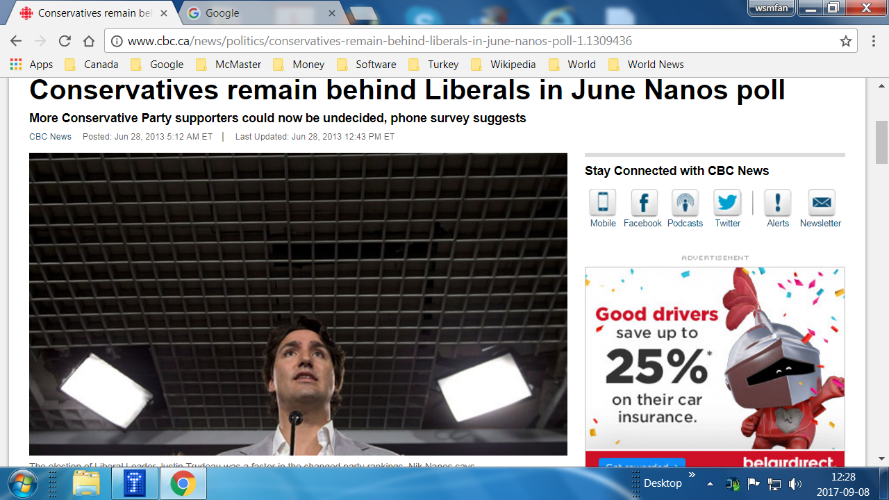
Statistics is everywhere! Do you see it even in this news item?

Nanos Poll (Justin T.) (.pdf)

As of mid-June 2013, Liberals had the support of 34.2% of voters, Conservatives 29.4%, and NDP 25.3%.
The article states that Nanos surveyed 816 committed voters and the poll is accurate plus or minus 3.5 percentage points, 19 times out of 20.
This is an example of Confidence Intervals. So, we are 95% sure that the true proportion of Liberal support is approximately somewhere between 30.7% (34.2 - 3.5%) and 37.7% (34.2 + 3.5%). [Technical note: The symmetric CI is valid only when the sample proportion is at 0.50.] We sometimes write the interval as [30.7,37.7].

(a) Topic 1: Installations / Introduction to R Graphics

a.1 Installations

As of 2017-05-05, current version for R is 3.4.0, and for Rcmdr 2.3-2.

a.1.1 Software Installation Videos

If you want to see and hear videos where I explain how to install R and R Commander software, please visit the following link:

The Install Videos . These videos show the installations of R and Rcmdr on PC and Mac computers.

a.1.2 Software Installation Documentation

If you want to follow written instructions, please see below.

Important! If you want to save your datasets and other files, please follow these instructions:

Before downloading any of the datasets, you should create a folder (preferably under "My Documents") and give it a name similar to the dataset.
Save your dataset to the folder you created.
After starting Rcmdr, click "File > Change Working Directory..." and point at the folder you have created for that dataset.
Any files you save from within Rcmdr will then appear in the folder you have created.

Instructions for downloading and installing R amd Rcmdr on Windows. [Link for downloading R.] Here are the screenshots for the steps to install R and Rcmdr:

First, uninstall earlier versions of R (if applicable):

Screenshots of step-by-step instructions to uninstall earlier version of R

Install R:

Screenshots of step-by-step instructions to install R

Install Rcmdr (from within R):

Screenshot of step-by-step instructions to install Rcmdr

Note: For R's Mac OS X and Linux/Unix installation instructions, please click here.

Note: For Rcmdr's Mac OS X and Linux/Unix installation instructions, please click here.

Wolfgang Jank's book Business Analytics for Managers (Use R!) may be useful in the core statistics course and it is available free-of-charge as a .pdf file from McMaster's online library.

The "theory" (i.e., background material) behind the techniques described below will be given after each example.

a.2 Graphics in R

Example: Let's use the Direct marketing data set [Table 2.6 DirectMarketing.csv] to plot some amazing graphs via Rcmdr. In this problem, we are trying to establish which age group should be targeted for increased revenues. Graphics obtained from Rcmdr in this dataset are here as a .pdf file.

We can also do a correlation plot of the above dataset using corrplot. Rcmdr first generates the correlation matrix which we call M and then ask corrplot to do the work. Here are the results.

Background material for graphics on Wikipedia.

Exercise: Now use this House price data set [Table 2.1 HousePrices.csv] and generate graphics as we did above. Graphics obtained from Rcmdr in this dataset are here.

Exercise: The problem statement for this Education Level/Gender/Income problem is here. You will need this Excel data file [Education-Gender-Income.xlsx] to import into Rcmdr and do the calculations.

Go to top of the page

(b) Topic 2: Descriptive Statistics and Probability Calculations

b.1 Symmetry, positively-skewed and negatively-skewed.

Symmetric distribution

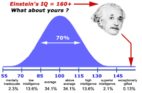
Example: Here is an Excel file [IQScores-1000.csv] of the IQ scores of 1,000 individuals. Plotting the histogram reveals that these scores are distributed in a symmetric manner. ¶

Mac salaries: Skewed or symmetric?

McMaster

Here's the distribution of the salaries of McMaster employees who earned above $100,000 in 2016. [McMaster-Salaries-2016.csv] Is the distribution symmetric, positively-skewed or negatively-skewed?

See if you can get the same results with the Excel version of this file: McMaster-Salaries-2016.xlsx. Hint: "Data > Import > From Excel file".

This information is public and the most recent data (for 2016 incomes) are available on the Ontario Government web site .

***

...and finally, an article which would interest almost everyone! The following link is excerpted from the book "Who We Are," by C. Rudder, 2014 (Random House), authored by the founder of OKCupid.com.

Dataclysm: The data guru for a popular dating site explains what men and women want from a mate (.pdf)

CAVEAT! The histogram for a "50-year old woman" above is somewhat biased. If the data were taken from OurTime.com, it would certainly look different. It may even be positively skewed.

An "outlier": Here is a news item about a 69-year old man and his 23-year old wife. (.pdf)

***

b.2 Mean and variance of a dataset

Example: I will motivate these concepts with the help of hot and cold water buckets!

Scenario 1: One bucket has freezing water at 0C, other has boiling water at 100C. Average is 50C. Why am I so uncomfortable?

Scenario 2: One bucket has lukewarm water at 50C, other has also lukewarm water at 50C. Average is 50C. So nice!

Both means are the same but what distinguishes the two scenarios? The Variance!

Example: (Exam scores in a small MBA class) Here is an Excel file of the calculations for mean and variance. If we have a population of N items, then division for variance is performed using N. If we have a sample of n items, then division for variance is performed using n-1.

Example/Exercise: Here is a .csv file of the same data. Use R to analyze it.

b.3 Probability calculations

coin toss

♦ Coin Toss : The fraction of heads obtained in a series of coin tosses approaches 0.5.

6-49

♦ Lotto 6/49 from Ontario Lottery Corporation. This is how they (used to) pick the six lucky numbers.

What is the probability of winning the big prize?

You have a better chance of being struck by lightning, but someone wins it. Look at this former DSB employee (.pdf).

What is the probability of winning in "Baby Lotto 2/4"?

NOTE: You can use the R command choose(4,2) to see how many combinations exist in the Lotto 2/4 game.
NOTE: The R command combn(4,2) lists all possible combinations.

---

♦ Birthdays : In a set of 50 randomly chosen people, what is the probability that any two will have the same birthday? Let's see what happened in our four sections.

Birthday

Birthdays in all four sections (Fall 2015)

The result may seem paradoxical; so, here's a link that explains the birthday problem.

Here, I explain this problem for the case of finding two matching birthdays as days of the week (M, T, W, Th, F, S, Su).

---

The Monty Hall Problem and Monty's show "Let's Make a Deal".

Monty asks: "Do you want to switch the door?"

Here are some explanations of this problem.

car and goats

Ron Clarke's explanation
Numb3rs Math
And here's a simulation page for this problem that works with Internet Explorer, only.
Here's my solution using a probability tree.

♦ We will talk about two important concepts (independence of events and mutually exclusive events) before the next Example.

♦ One final example: Psy's Gangnam Style on my iPod. What is the probability of getting Psy's song if I shuffle once? Shuffle three times? See notes.

Would you believe it? Even the Mac president (Dr. Patrick Dean) did the Gangnam Style dance (see 1:40).

Go to top of the page

(c) Topic 3: Random Variables

c.1 Discrete random variables

Example: Pierik's bikes. We will calculate the expected (mean) value of demand, E(X); and variance of demand Var(X).

Here is the Excel-based calculations of the mean demand and variance and s.d. of demand.

bicycle pierik

c.2 Binomial (a special discrete random variable)

Here is my handwritten notes on the binomial distribution.

balls Three tennis balls : My success probability at each throw is p = 0.6. What is the probability that I will have all three balls in the bucket? Two balls? One ball? Zero?

R documentation for binomial distribution.
Background material for binomial probabilities. Wikipedia.

Exercise: Here is a more challenging problem from healthcare area involving the testing of a new drug. Find the solution using Rcmdr. (Answer: 0.74)

*****

c.3 Normal (a special continuous random variable)

Example: Here is again the Excel file [IQScores-1000.csv] of the IQ scores of 1,000 individuals. Plotting the histogram and other related graphs, especially the Quantile comparison plot, reveal that these scores are distributed normally with a mean of about 100 and a standard deviation of about 15. The probability that someone picked at random from this group has an IQ of at least 145 is 0.0013. Here are the results. ¶

More examples:

Normal distribution

Heights (in meters) and handspans (in centimeters) of students. Here is what everyone wrote:

Actual height and handspan data (2015) [.xlsx]
And here is the .csv file to analyze with R.
For the group of females, we have, approximately, mean = 1.65 meters and s.d. = 0.06 meters. Check to see that the empirical rule works well here.

Exam marks : Normally distributed exam marks of a large class (475 students) from a few years ago. An easy method for checking normality is the normal curve plot: If it looks linear, then the data must be normal.

Binomial and normal : When n is large and p is around 0.5, binomial looks like normal. The next few links illustrate this.

Galton's Board: Here's what happens if you drop a large number of marbles in the board and p = 1/2. (Binomial turns into normal.) This link does it in real time. But here is a cool animation.

Check this out to see how the shape of the normal distribution changes if we vary the mean and standard deviation.

Visual check for normality: We will do this with R's "Quantile comparison plot" (under Graphs). The graphs should look like a straight line as it does for Exam marks data.

Here is a Wikipedia article on the normal distribution.

---

c.4 An important example (Roulette)

♦ Roulette is a board game with a large "house edge."

Here is the board for American roulette:

The roulette wheel looks like this: Wheel

Payout amounts if you win your bet in roulette. (Accessible from Avenue.)

This link simulates the roulette game.

But please note: I am not advocating gambling; in fact, I am very much against playing such games as they eventually ruin the gambler. The purpose of this example is to illustrate that roulette is an unfair game and you shouldn't play it with real money!

What is the probability of winning if you bet,

On Red? (If you bet $1 and you win, you get $1)
On 1st 12? (If you bet $1 and you win, you get $2)
On 17? (If you bet $1 and you win, you get $35)

We will do a few examples.
Warning! In the long run, your winnings are always less than the amount you bet. SO, IF YOU KEEP PLAYING, YOU WILL LOSE EVERYTHING YOU HAVE!
Why would you want to buy a stock which will surely lose you money in the long run?

The expected value in American Roulette is -5.2%. That is, every time you bet $100, on average you LOSE $5.2.

Go to top of the page

(d) Topic 4: Confidence Intervals and Hypothesis Testing

d.1 Confidence intervals

Poll Results

Poll

Nanos Poll

Return to the polling example.
As of mid-June 2013, Liberals had the support of 34.2% of voters, Conservatives 29.4%, and NDP 25.3%.
The article states that Nanos surveyed 816 committed voters and the poll is accurate plus or minus 3.5 percentage points, 19 times out of 20.
So, we are 95% sure that the true proportion of Liberal support is approximately somewhere between 30.7% (34.2 - 3.5%) and 37.7% (34.2 + 3.5%).
There is a formula to find how 816 is obtained if desired "error" is plus or minus 3.5%.

Confidence Intervals for the Proportion p

We will do this with the participation of the class and we will use an inflatable globe to estimate the proportion of the water surface to the total surface of the globe.

Here is the video of this experiment I recorded in Section C02 (November 4, 2010, Thursday).

*****

Example: (Population proportion) The CI for population proportion is easy to obtain. Suppose you poll 1000 people and 340 of them state that they would vote Liberal, if the election were held today. Here is what we do to find a 95% CI:

> prop.test(340,1000)

1-sample proportions test with continuity correction

data: 340 out of 1000, null probability 0.5
X-squared = 101.761, df = 1, p-value < 2.2e-16
alternative hypothesis: true p is not equal to 0.5
95 percent confidence interval:
0.3108142 0.3704312
sample estimates:
p
0.34

So, the sample proportion is 0.34, with a 95% CI of [0.3108,0.3704], i.e., a margin of error of about 3%. ¶

R documentation for prop.test.
Background material for confidence interval for population proportion. Wikipedia.

Example: Here is an hypothetical problem. One thousand US citizens were asked who they would vote for; Trump or Clinton? The sample results are in this Excel file [Trump-vs-Clinton.xlsx]. What is the CI for Clinton supporters? We use Rcmdr's single-sample proportion test, and obtain these results. Note that this test works with text data as "factors," only. ¶

Exercise: Find a 99% CI for the population proportion problem (Liberal supporters) discussed above. You will need to refer to the R documentation for prop.test to do this.

d.2 Hypothesis testing

"Hypo-thesis" is something that is yet to be proven to be true.)

Lady

"The Lady Tasting Tea" : Can tea poured into milk taste differently than that of milk poured into tea? This experiment was originally designed by Professor Ronald Fisher and it will help us motivate the discussion of hypothesis testing. We will, however, use Coke and Pepsi in our experiment.

In case you were wondering, here is the mathematics behind the calculations. In this link you can find the probaibilities of 0, 2, 4, 6 or 8 correct identifications which uses the hypergeometric probabilities (which we did not discuss).

Type I and Type II errors

Steven

Type I error : In 1959, Steven Truscott was found guilty of murdering his classmate even though he did not commit any crime. In 2007, he was formally acquitted of the crime. In 2008, the government of Ontario awarded him $6.50 million in compensation

Type II error : Many people believe that O. J. Simpson had murdered his wife and he should have been found guilty. But after a lenghty trial, he was acquitted in 1995.

Examples

Hypothesis testing in R (with one or two populations) still uses the t.test function described above. We now discuss a problem with one population.

Example: The data set [Atkins-Diet.csv] concerns the weight losses experienced by dieters using the Atkins diet. We want to test Atkins's hypothesis that people who use their method lose, on average, at least 20 pounds in 6 months. The p-value is about 0.03 so we reject this hypothesis. However, if the claim is at least 10 pounds in 6 months, we find p-value as 0.98, so we don't have enough evidence to reject this claim. Here are the results from Rcmdr. ¶

R documentation for t.test.
Background material for hypothesis testing. Wikipedia.

Exercise: For the Atkins problem test the null hypothesis that Atkins users lose, on average, 17 pounds after 6 months. (This is now a two-sided test.)

Exercise: Use the following data values to test the hypothesis that true mean is 750 vs. the hypothesis that it differs from 750: (801,814,784,836,820) What is the p-value? (Answer: p = .0023; so reject the null)

Go to top of the page