Session 1. Introduction to R and R
Commander (Rcmdr) and R functions for basic statistical models
Statistics is everywhere! Do you see it even in this news item?
Nanos
Poll
- As of mid-June 2013, Liberals had the support of 34.2% of voters,
Conservatives 29.4%, and NDP 25.3%.
- The article states that Nanos surveyed 816 committed voters and the
poll is accurate plus or minus 3.5 percentage points, 19 times out of
20.
- This is an example of Confidence
Intervals.
(a) Preliminaries
Instructions for downloading and installing R amd Rcmdr on Windows. [Link for downloading R.]
Here are the screenshots for the steps to install R and Rcmdr:
First, uninstall earlier versions of R (if applicable):
Screenshots of step-by-step instructions to uninstall earlier version of R
Install R:
Screenshots of step-by-step instructions to install R
Note 1: After the "Select Additional Tasks" window, R will install several files on your computer.
Note 2: After "Completing the R for Windows ..." window, R is installed on your computer. Now go to your desktop and choose "Run as adminstrator" on the R icon.
Install Rcmdr (from within R):
Screenshot of step-by-step instructions to install Rcmdr
Note: For R's Mac OS X and Linux/Unix installation instructions, please click here.
Note: For Rcmdr's Mac OS X and Linux/Unix installation instructions, please click here.
As of 2016-06-16, current version for R is 3.3.0, and for Rcmdr 2.2-4.
*
We will be using Wolfgang Jank's book Business Analytics for Managers (Use R!) in Session 2 which can be purchased from amazon.com. Or, it may be available at your school's online library as a .pdf file.

(b) R functions
The "theory" (i.e., background material) behind the techniques described below will be given after each example.
b.1 Graphics in R

Example: Let's use the Direct marketing data set [Table 2.6 DirectMarketing.csv] to plot some amazing graphs via Rcmdr. Graphics obtained from Rcmdr in this dataset are here as a .pdf file.
We can also do a correlation plot of the above dataset using corrplot. Rcmdr first generates the correlation matrix which we call M and then ask corrplot to do the work. Here are the results. 
-
- Background material for graphics on Wikipedia.
Exercise: Now use this House price data set [Table 2.1 HousePrices.csv] and generate graphics as we did above. Graphics obtained from Rcmdr in this dataset are here.
Exercise: The problem statement for this Education
Level/Gender/Income problem is here. You will need this Excel data file [Education-Gender-Income.xlsx] to import
into Rcmdr and do the calculations.
b.2 Probability calculations
Binomial distribution

Example: Historical records indicate that 40% of all customers who enter a discount store make a purchase. What is the probability that two of the next three customers will make a purchase?
This is a binomial problem. The result is 0.288 as shown in this file. This is obtained in Rcmdr via the steps, Distributions > Discrete Distributions > Binomial Distribution > ... Try to replicate the results. 
Exercise: Here is a more challenging problem from healthcare area involving the testing of a new drug. Find the solution using Rcmdr. (Answer: 0.74)
*****
Normal distribution
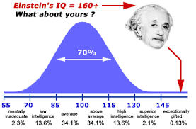
Example: Here is an Excel file [IQScores-1000.xlsx] of the IQ scores of 1,000 individuals. Plotting the histogram and other related graphs, especially the Quantile comparison plot, reveal that these scores are distributed normally with a mean of about 100 and a standard deviation of about 15. The probability that someone picked at random from this group has an IQ of at least 145 is 0.0013. Here are the results. 

Example: Distribution of fuel efficiencies of a new model car, X, is normal. Assuming that X ~ N(7.13,0.27^2) find the probability Pr(6.75 < X < 7.49). Here is the result from Rcmdr. 
Exercise: Weekly demand at a grocery store for a particular brand of energy drink cans is N(1000,100^2). How many cans should be stocked so that there is a 5% chance of a stockout? (Answer: 1165 cans)
b.3 Confidence intervals

Example: (Population mean) A company's financial health is (usually) measured using its debt-to-equity ratio. A bank has collected n = 15 of its commercial accounts in this file [DebtEq.csv]. Let's find the 95% confidence interval (CI) using Rcmdr. (This is done via the t-test command which includes the CI. Here is the result. 
Exercise: In the debt-to-equity ratio problem discussed above, use the same dataset [DebtEq.csv] to find a 90% CI.
Exercise: Let's find a 95% CI for the true average weight of SlimPhone. The population s.d. is known to be 0.6 gr. We take a sample of n = 5, and find the sample mean as 70.12 gr. Note: Here we don't have any dataset; just the sample mean. (Answer: [69.594,70.646])
*****

Example: (Population proportion) The CI for population proportion is easy to obtain. Suppose you poll 1000 people and 340 of them state that they would vote Liberal, if the election were held today. Here is what we do to find a 95% CI:
> prop.test(340,1000)
1-sample proportions test with continuity correction
data: 340 out of 1000, null probability 0.5
X-squared = 101.761, df = 1, p-value < 2.2e-16
alternative hypothesis: true p is not equal to 0.5
95 percent confidence interval:
0.3108142 0.3704312
sample estimates:
p
0.34
So, the sample proportion is 0.34, with a 95% CI of [0.3108,0.3704], i.e., a margin of error of about 3%. 
Example: Here is an hypothetical problem. One thousand US citizens were asked who they would vote for; Trump or Clinton? The sample results are in this Excel file [Trump-vs-Clinton.xlsx]. What is the CI for Clinton supporters? We use Rcmdr's single-sample proportion test, and obtain these results. Note that this test works with text data as "factors," only. 
Exercise: Find a 99% CI for the population proportion problem (Liberal supporters) discussed above. You will need to refer to the R documentation for prop.test to do this.
b.4 Hypothesis testing
Hypothesis testing in R (with one or two populations) still uses the t.test function described above. We now discuss a problem with one population.

Example: The data set [Atkins-Diet.csv] concerns the weight losses experienced by dieters using the Atkins diet. We want to test Atkins's hypothesis that people who use their method lose, on average, at least 20 pounds in 6 months. The p-value is about 0.03 so we reject this hypothesis. However, if the claim is at least 10 pounds in 6 months, we find p-value as 0.98, so we don't have enough evidence to reject this claim. Here are the results from Rcmdr. 
Exercise: For the Atkins problem test the null hypothesis that Atkins users lose, on average, 17 pounds after 6 months. (This is now a two-sided test.)
Exercise: Use the following data values to test the hypothesis that true mean is 750 vs. the hypothesis that it differs from 750: (801,814,784,836,820) What is the p-value? (Answer: p = .0023; so reject the null)
b.5 ANOVA
The final example involves analysis of variance (ANOVA) where we want to test the null hypothesis that three or more population means are equal. Once again, Rcmdr solves this problem quite admirably.

Example: (One-way ANOVA) Let's consider a problem from agricultural testing in an experimental farm. We want to test the null hypothesis that low (L), medium (M) or high (H) fertilizer levels do not differ in their effects on the average yield of a new plant. We have 18 small plots, and on six randomly selected plots we use L, the other six M and the last six H. Here is the data set [Fertilizer.csv] for this example. Rcmdr uses the R function aov and finds these results. 
Exercise: Refer to your
favourite statistics text for a solved problem on one-way ANOVA. Use the steps above to check the solution.
Exercise: Use this hypothetical dataset with four samples (A, B, C, and D) to do a one-way ANOVA on the equality of the means. What is the p-value? (Answer: p = 0.00146, so reject the null)
*****

Example: (Two-way ANOVA) Note that the above example is a one-factor ANOVA problem. R can of course deal with multi-factor problems, too. Consider the data in this file [BakeSale2-For-R.csv] where we have two factors: Shelf display height (Bottom, Middle, Top) and shelf display width (Regular, Wide). The numbers in each cell correspond to sample group means (sales) for the last six months from three different stores. This is a 2 x 3 (or, 3 x 2) design.
We want to test three hypotheses: (i) There is no interaction between the factors, (ii) Factor 1 (height) has no effect on sales, (iii) Factor 2 (width) has no effect on sales. These results show that (i) little or no interaction exists between height and width (high p-value), (ii) height affects the sales (p-value near zero), (iii) width does not affect sales (high p-value). Here, the p-values are denoted by Pr(F>). 
Exercise: Refer to your
favourite statistics text for a solved problem on two-way ANOVA. Use the steps above to check the solution.
Exercise: Use this dataset with two factors (gender and machine type possible affecting productivity) to test the hypotheses. As before, there will be an F-ratio for each factor and also for the interaction. It may be that there is no difference between Male and Female, or between machines A and B. But if men do better on machine B and women do better on machine A, then there will be interaction. (Answer: In fact, you will notice that there is no difference between genders and the machines, but there is a Gender:Machine interaction with a very low p-value.)