 vs.
vs. 
Example: Let's use the sales and advertising data and analyze it.
In this section we will look at sales/advertising/income data and consider simple and multiple linear regression models.
 vs.
vs. 
Example: Let's use the sales and advertising data and analyze it.
Exercise: Consider this house price dataset for 124 houses. Do a simple regression with Price as dependent variable and SqrFt as independent variable. Perform analysis similar to what we did above with the advertising/sales problem. (Answer: Regression equation is Price = 259.88 + 120.16 x SqrFt.)
 vs.
vs.  and
and 
Example: Now we use the sales vs. advertising and income data. So, this is a multiple regression problem which is solved as follows:
Exercise: Consider the same house price dataset for 124 houses used above. Now use SqrFt, LotSize, Bedrooms and Bathrooms as independent variables and Price as dependent variable and perform a multiple regression.

Example: This is a more challenging problem with qualitative factors (such as Yes/No, North/West/East) for some variables in the dataset. To find the regression equation, you will need to use Rcmdr's Statistics > Fit Models > Linear Model as LinearModel.1 <- lm(Price ~ Bathrooms + Bedrooms + Brick + Neighborhood + Offers + SqFt, data=Dataset). The confint(LinearModel.1) command will produce the confidence intervals for coefficients. Here are the results.
Dummy variables are needed when some of the variables assume binary values. Including interaction terms aid the analyst to obtain more accurate results in regression.

Example: Let's consider the dataset for salaries. When we ignore the gender and plot the dataset, we are missing out on the information inherent in the gender differences. Only when we plot the data according to gender group, we see a more clear picture. The Rcmdr results are here. So, if we just consider the Experience and Salary columns, the regression equation is found as Salary = 59033.1 + 1727.3 x Experience. But is this accurate?
*****
Example: Here, we need to use a dummy variable to distinguish between males and females. We define Gender.Male = 1 if gender is "male" and 0 otherwise. The new dataset with this information is here. Using RegModel.3 <- lm(Salary~Experience+Gender.Male, data=Dataset), we find Salary = 53260.0 + 1744 x Experience + 17020 x Gender.Male. (R-squared = 0.31.)
Note: Of course, there is an easier way to do this with Rcmdr without using the Gender.Male construct. Just use the "Linear model". Rcmdr knows that Gender is a factor. If you pick it as an independent variable, R figures out the rest and you get the same result as Salary = 53260 + 1744 x Experience + 17020 x Gender[T.Male].
Exercise: Use this dataset to estimate the travel time given, (i) distance travelled, (ii) number of deliveries and (iii) truck type. Note that truck type is a factor here and Rcmdr recognizes it. (Answer: 0.5222 + 0.0464 x Km + 0.7102 x Deliveries + 0.9 x TruckType[T.Van].)

Example: We noted above that each additional year of experience is 1,744 for either gender. But this is not quite logical. Could it be more for males? We analyse this using an interaction term in the form Gender.Exp.Int = Gender.Male x Experience. The dataset with the interaction term is here. The regression equation is obtained as Salary = 66,333 + 666 x Experience - 8,034 x Gender.Male + 2,086 x Gender.Exp.Int. (R-squared = 0.55.)
Now what happens?
Note 1: Of course, as before, there is an easier way to do this with Rcmdr without using the Gender.Exp.Int construct. Just use the "Linear model" and incorporate the product of Gender and Exp as a new variable. Rcmdr figures out what to do and finds exactly the same result. You can do this as an Exercise.
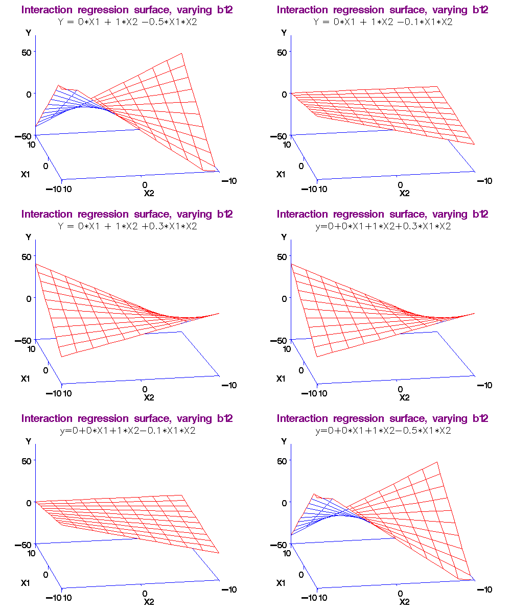
Note 2: What exactly do we mean by "interaction." I will make this more clear in the workshop by comparing two functions: (i) f(x,y) = ax + by, and (ii) f(x,y) = ax + by + cxy. In the first case, there is no interaction between x and y, but in the second there is! (Just find the partial derivative of f(x,y) w.r.t. variable y in both cases and you will see the difference.)

Is it always a good idea to include as many independent variables as we can in a regression problem? No! Let's see why.
Example: Consider the dataset for a problem with sales and assets as independent variables and profit as the dependent variable.
Exercise: Use this dataset to find a regression equation for Time as dependent variable and Km, Deliveries and Gas (consumed) as independent variables. Is there a high correlation between Km and Gas? What can go wrong with such problems?
R has a nice way of dealing with the multicollinearity problem using stepwise regression.
Example: We use the same dataset as above. The stepwise procedure is applied after the regression problem is solved by using Models > Stepwise Model Selection... Here is the result.
Exercise: Consider again the house price dataset for 124 houses. Run a regression with Price as the dependent variable and everything else (except SubDiv) as independent variable. Next, use Models > Stepwise Model Selection... and reduce the model with Akaike Information Criterion (AIC) and the backward/forward direction. How many independent variables do you have left and what is the AIC? (Answer: We have 5 variables left as Price ~ Bathrooms + Bedrooms + Distance + LotSize + SqrFt, and AIC is 736.41.)