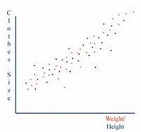
 vs.
vs. 
Here is a cool animation for finding the regression line: Animation for regression
Example: Let's use the sales and advertising data [Table3.1Sales-Advertising.csv] and analyze it.
In this section we will look at sales/advertising/income data and consider simple and multiple linear regression models.
 vs.
vs. 
Here is a cool animation for finding the regression line: Animation for regression
Example: Let's use the sales and advertising data [Table3.1Sales-Advertising.csv] and analyze it.
Example (Added after the workshop) : Here's an amazing example of four problems with very diffrent datasets which give the same results. Anscombe's quartet.
Exercise: Consider this house price dataset [HousePrices-Data.csv] for 124 houses. Do a simple regression with Price as dependent variable and SqrFt as independent variable. Perform analysis similar to what we did above with the advertising/sales problem. (Answer: Regression equation is Price = 259.88 + 120.16 x SqrFt.)
 vs.
vs.  and
and 
Example: Now we use the sales vs. advertising and income data [Table 3.1 Sales-Advertising-Income.csv]. So, this is a multiple regression problem which is solved as follows:
Exercise: Consider the same house price dataset [HousePrices-Data.csv] for 124 houses used above. Now use SqrFt, LotSize, Bedrooms and Bathrooms as independent variables and Price as dependent variable and perform a multiple regression.

Example: This is a more challenging problem with qualitative factors (such as Yes/No, North/West/East) for some variables in the dataset [Table2.1HousePrices.csv]. To find the regression equation, you will need to use Rcmdr's Statistics > Fit Models > Linear Model as LinearModel.1 <- lm(Price ~ Bathrooms + Bedrooms + Brick + Neighborhood + Offers + SqFt, data=Dataset). The confint(LinearModel.1) command will produce the confidence intervals for coefficients. Here are the results.
Prediction of the dependent variable when factors are present (such as Brick, Neighboorhood) can be a little tricky. Here is what you need to do if you want to predict the price of a house with 2 bathrooms, 5 bedrooms, brick, north neighborhood, 2 offers and 1000 sqft. As usual, the highlighted commands are entered manually.
I used the corrplot package to plot the correlations between different numerical variables in this example. Here is the result. 
Example (Added after the workshop) : How long would it take to generate 1,000,000 observations (standard normal) for 100 variables plus the means? Once that is done, how long does it take to run a 100 independent variable multiple regression problem with the 1,000,000 observations? (Just a minute or two!) We will do this in class.
Exercise: The problem statement for this Education Level/Gender/Income problem is here. You will need this Excel data file [Education-Gender-Income.xlsx] to import into Rcmdr and do the calculations.
Dummy variables are needed when some of the variables assume binary values. Including interaction terms aid the analyst to obtain more accurate results in regression.

Example: Let's consider the dataset for salaries [Table4.1GenderDiscrimination.csv]. When we ignore the gender and plot the dataset, we are missing out on the information inherent in the gender differences. Only when we plot the data according to gender group, we see a more clear picture. The Rcmdr results are here. So, if we just consider the Experience and Salary columns, the regression equation is found as Salary = 59033.1 + 1727.3 x Experience. But is this accurate? 
*****
Example: Here, we need to use a dummy variable to distinguish between males and females. We define Gender.Male = 1 if gender is "male" and 0 otherwise. The new dataset with this information is here [Table4.1GenderDiscrimination-Dummy.csv]. Using RegModel.3 <- lm(Salary~Experience+Gender.Male, data=Dataset), we find Salary = 53260.0 + 1744 x Experience + 17020 x Gender.Male. (R-squared = 0.31.)
Note: Of course, there is an easier way to do this with Rcmdr without using the Gender.Male construct. Just use the "Linear model". Rcmdr knows that Gender is a factor. If you pick it as an independent variable, R figures out the rest and you get the same result as Salary = 53260 + 1744 x Experience + 17020 x Gender[T.Male].
Exercise: Use this dataset [Butler-x1-x2-Dummy.csv] to estimate the travel time given, (i) distance travelled, (ii) number of deliveries and (iii) truck type. Note that truck type is a factor here and Rcmdr recognizes it. (Answer: 0.5222 + 0.0464 x Km + 0.7102 x Deliveries + 0.9 x TruckType[T.Van].)

Example: We noted above that each additional year of experience is 1,744 for either gender. But this is not quite logical. Could it be more for males? We analyse this using an interaction term in the form Gender.Exp.Int = Gender.Male x Experience. The dataset with the interaction term is here [Table 4.1 Gender Discrimination-Recode-Interaction.csv]. The regression equation is obtained as Salary = 66,333 + 666 x Experience - 8,034 x Gender.Male + 2,086 x Gender.Exp.Int. (R-squared = 0.55.)
Now what happens?
Note 1: Of course, as before, there is an easier way to do this with Rcmdr without using the Gender.Exp.Int construct. Just use the "Linear model" and incorporate the product of Gender and Exp as a new variable. Rcmdr figures out what to do and finds exactly the same result. You can do this as an Exercise. 
Note 2 (Added after the workshop): There is an even easier way to get the same results. Just enter Gender=="Male" in the subset box in Linear model, and R gives the regression results for males, only. You can do this as an Exercise. 
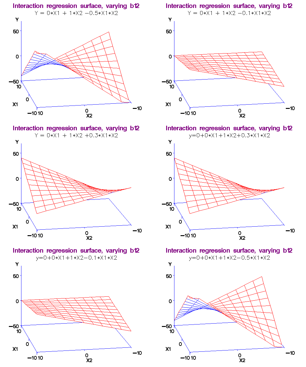
Note 3: What exactly do we mean by "interaction." I will make this more clear in the workshop by comparing two functions: (i) f(x,y) = ax + by, and (ii) g(x,y) = ax + by + cxy. In the first case, there is no interaction between x and y, but in the second there is!
Here's why: df/dx = a, so that df = a*dx, i.e., the changes in y do not affect f in this case.
But for the second function, dg/dx = a + cy, so that dg = (a + cy)*dx, i.e., changes in y do affect g!
Note 4: Here are some real-life examples of interaction from Wikipedia.
Example: In every model we discussed, we assumed that the relationship between the independent variable(s) and the dependent variable was essentially linear. This allowed us to use linear regression. But, what if the relationship is not linear? Does using linear regression produce inaccurate results? In fact, it does, and we need to revise our approach to solving such problems.
To illustrate, consider this dataset [Table2.6DirectMarketing.csv] where we examine the relationship between Salary and AmountSpent variables. In this output, we first look at the scatterplot and do a simple regression. The data seem to be approximating a funnel, and we get poor results with an R^2 = 0.4894. Next, we transform both variables using logarithms, and this gives a better looking scatterplot. Running the regression, we find R^2 = 0.5816. We suspect that the AmountSpent also depends on the Location variable (as seen in the new scatterplot), so we include Location as a factor and obtain even better results with R^2 = 0.645.
The interpretation of the estimates of the coefficients will be provided in the next simple example.
But, first a bit of "theory."
Suppose you are not convinced that a linear relationship between price (P) and demand (D) is justifiable; so you decide to use a nonlinear one, e.g., D = exp(a)*P^b where a and b are your coefficients. If you differentiate both sides, we get
dD/dP = exp(a)*b*P^(b-1) = b*exp(a)*P^b*(1/P) = b*D/P.
Rewriting, we have,
dD/D = b*dP/P,
which says that if you increase price P by 1%, demand D will change by b%. (For example, if P = 100, dP = 1, then dP/P = 1%. Now, if b = -2.5, this means that dD/D = -2.5%, so demand will go down by 2.5%.)
Now, taking the logarithms of both sides of D = exp(a)*P^b, we get log(D) = a + b*log(P), which is a nice linear equation, if you write y = log(D) and x = log(P). This means that we can do whatever we were doing as before on the log transformed problem and use the results keeping in mind the meaning of the coefficient b. This is what we will do next. 
Example (Added after the workshop) : Here is a fascinating example with dataset from the United Nations on a country's GDP and the infant mortality. (The data file is in native R format, i.e., it is not an Excel file.) The data is highly nonlinear and a linear fit gives terrible results. But a log transformation of both variables produces a reasonably linear cloud of points through which we fit a line quite accurately. Here are the results. 
Example: Let's consider this data set [Table 4.2 PriceAndDemand.csv] for this example. The scatterplot reeals that there may be a nonlinear relationship between price and quantity. Initially, we fit a line to the data and obtain an R^2 = 0.6236. The graphs obtained for the model reveal that the assumption of errors being normal is not satisfied. When we further do a scatterplot with log x and log y axes, the graph of transformed data appears more linear. A fit using log(Price) and log(Qty) gives the coefficient b = -1.1810 which means that for a 1% increase in price, quantity demanded would reduce by about 1.181%. Here is the output of the results. 

Is it always a good idea to include as many independent variables as we can in a regression problem? No! Let's see why.
Example: Consider the dataset [Table5.1Sales-and-Assets.csv] for a problem with sales and assets as independent variables and profit as the dependent variable.
Exercise: Use this dataset [Butler-x1-x2-Multicollinear.csv] to find a regression equation for Time as dependent variable and Km, Deliveries and Gas (consumed) as independent variables. Is there a high correlation between Km and Gas? What can go wrong with such problems?
R has a nice way of dealing with the multicollinearity problem using stepwise regression.
Example: We use the same dataset [Table5.1Sales-and-Assets.csv] as above. The stepwise procedure is applied after the regression problem is solved by using Models > Stepwise Model Selection... Here is the result.
ASSIGNMENT: Consider again the house price dataset [HousePrices-Data.csv] for 124 houses.